Particle Propagation in the Heliosphere
Introduction
The propagation of relativistic charged particles in the heliosphere and interstellar magnetic fields is calculated using the ptracing code. This code was originally developed for the studies described in Desiati & Zweibel (2014). It includes several analytical magnetic and electric field configurations and interfaces to different heliospheric numerical models. Additionally, it supports multithreading, allowing it to take full advantage of computers with a large number of CPU cores and shared memory.
Trajectories are calculated by numerically integrating the following set of 6–dimensional ordinary differential equations
$$\frac{d\mathbf{p}}{dt} = q \left(\mathbf{v}\times\mathbf{B} \right), \, \frac{d\mathbf{r}}{dt} = \mathbf{v},$$describing the Lorentz force exerted by the magnetic field $\mathbf{B}(\mathbf{r})$ on particles with electric charge $q$ and velocity $\mathbf{v}$, where $\mathbf{r}$ is their position vector and $\mathbf{p}$ the momentum. Momentum is expressed in units of $mc$; $\hat{\mathbf{p}}\equiv\mathbf{p}/mc$. The particle velocity $\mathbf{v}$ is related to $\hat{\mathbf{p}}$ by $\mathbf{v} = \hat{\mathbf{p}}/\sqrt{1+\hat p^2}$ and the particle Lorentz factor $\gamma = \sqrt{1+\hat p^2}$. In these units, the dimensionless particle gyroradius is $\hat r_g = \hat p_{\perp}$, and the dimensionless gyro-frequency is $\hat \omega_g = 1/\gamma$. %We denote normalized variables with a hat.
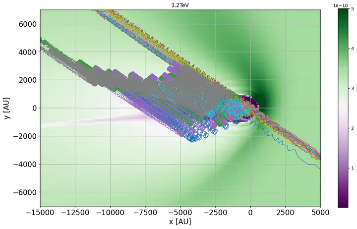
The equations of motion can be numerically integrated using various stepping algorithms. The code supports an adaptive time step size in these calculations, with a tolerance level denoted by a parameter $\epsilon$ to ensure that truncation errors remain sufficiently small. The integration of particle trajectories concludes when either the maximum integration time, $t_\mathrm{max}$, is reached or when the particles have attained a radius of $r_\mathrm{max}$. The figure demonstrates how protons are affected by the heliosphere and the modified magnetic field near its boundary.
One challenge in calculating trajectories within open boundary systems is that particles propagating from outside the heliosphere have a very low probability of reaching Earth or passing near it. To address this, we plan to generate 100 million anti-proton trajectories, propagating backward from Earth to a distance of 50,000 AU from the Sun.
We compute the trajectories using the Boris Push stepping method. This algorithm has become a standard for this purpose. Although the Boris algorithm is not symplectic, it does conserve phase space volume, and its energy error is globally bounded, comparable to that of symplectic algorithms. To ensure the accuracy of our results and as part of our validation procedure, we will perform additional checks by varying the integration tolerance parameters and comparing the outcomes with the explicit fourth-order Runge-Kutta method. Additionally, we will conduct cross-validation with limited statistics using third-party tools such as CRPropa.
We calculate trajectories using heliospheric models provided by our collaborator, Prof. Nikolai Pogorelov, to investigate the systematic effects of model parameters on our data interpretation. According to Liouville’s Theorem, we can interpret the calculated back-propagated anti-proton trajectories as protons traveling from the ISM to Earth.
Experimental biases on the heliospheric contribution to the observed TeV cosmic ray anisotropy
A preliminary study utilized numerically computed particle trajectories from a computational heliospheric model to assess the experimental biases introduced by ground-based experiments and their impact on interpretations. We intend to conduct thorough investigations into this experimental dimension of cosmic-ray physics, which will aid in developing the analytical tools needed to explore the origins of cosmic-ray anisotropy and its propagation through the interstellar medium and the heliosphere.
The paper examines how the heliosphere acts as a magnetic lens that reshapes the TeV cosmic-ray anisotropy we observe on Earth, complicating efforts to infer the true interstellar distribution. Because ground-based reconstructions are effectively “blind” to the north–south (m=0) spherical-harmonic terms, the vertical component of the dipole is lost, which can bias estimates of the pitch-angle distribution in the local interstellar medium (LISM). Even so, the paper argues that higher-order multipoles preserve enough spatial information to constrain the large-scale structure and its alignment with the local interstellar magnetic field (LIMF). The premise is that if we correctly model the heliospheric imprint and account for observational limitations, we can still recover the underlying LISM anisotropy.
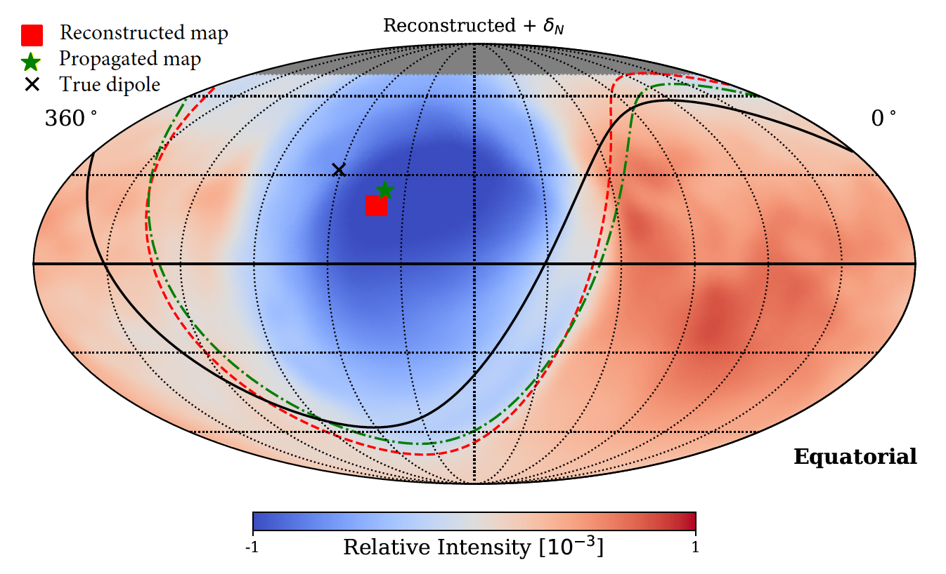
Using back-propagation through a heliospheric field model across multiple rigidities, we reconstruct Earth-frame sky maps, fit the boundary between excess and deficit to infer the LIMF “magnetic equator,” and estimate the missing north–south dipole component. Remapping the result outside the heliosphere then yields an interstellar dipole whose direction is within about 3° of the true LIMF when that compensation is applied (versus ~14° without it). At ~10 TV rigidity, where particle gyroradii match the LIMF draping scale, the heliospheric effect is strong but does not destroy the overall ordering with the LIMF; the method’s accuracy, however, depends on the chosen heliosphere/LIMF model. The paper highlights the next steps, which include scanning heliotail length, solar-cycle phase, turbulence, and LIMF geometry to quantify model sensitivities.
Chaotic Behavior of Trapped Cosmic Rays
A recently published paper develops a practical way to quantify how cosmic rays behave chaotically when they’re temporarily trapped by coherent magnetic structures—especially the heliosphere acting as a magnetic mirror. Using an axially symmetric “magnetic bottle” tailored to heliospheric scales (field strengths ~1–3 μG; mirror separation ~2000 au), the authors integrate ensembles of 1 TeV test-particle trajectories and compute finite-time Lyapunov exponents (FTLEs), which measure how rapidly nearby trajectories diverge over a chosen time window. They also add time-dependent perturbations designed to mimic solar-cycle polarity reversals (including a check on induced electric fields) to see how temporal variability alters the chaos. The key diagnostic is the joint behavior of FTLE versus a particle’s escape time from the mirror.
The central result is a robust power-law correlation: once particles have reached their most chaotic state, the FTLE scales approximately as the inverse of the escape time (slope ≈ −1), and this relation persists under weak and strong time perturbations. On that basis, trajectories naturally fall into regimes—transient (quick escape, little chaos), intermediate (brief explosive divergence), a broad “power-law” class (regular vs. irregular chaotic orbits with steadily increasing dwell times), and, in the unperturbed case only, long-lived trapped orbits. Mapping FTLE and escape time onto the sky reveals distinct regions and gradients in chaoticity; adding perturbations erases the strictly trapped region and redistributes particles toward shorter escape times, while maintaining the same FTLE–escape-time slope. Because 1–10 TV rigidities have gyroradii comparable to heliospheric scales, the study argues that chaotic mirroring can imprint time variability—on solar-cycle timescales and in specific sky sectors—on observed TeV anisotropy maps, such as those from HAWC+IceCube. The method provides a framework for interpreting such variations and is intended to be applied to more realistic MHD–kinetic heliosphere models and to other magnetic mirrors (e.g., superbubbles), thereby linking microphysical trajectory chaos to macroscopic anisotropy morphology.
The Role of the Heliosphere in Shaping the Observed Cosmic Ray Spectral Anisotropy
Report on a study of cosmic-ray tracing through the heliosphere to investigate the induced modulations in the energy spectrum of the cosmic rays. The work was presented at the ICRC 2025 Conference in Geneva.