Anisotropy

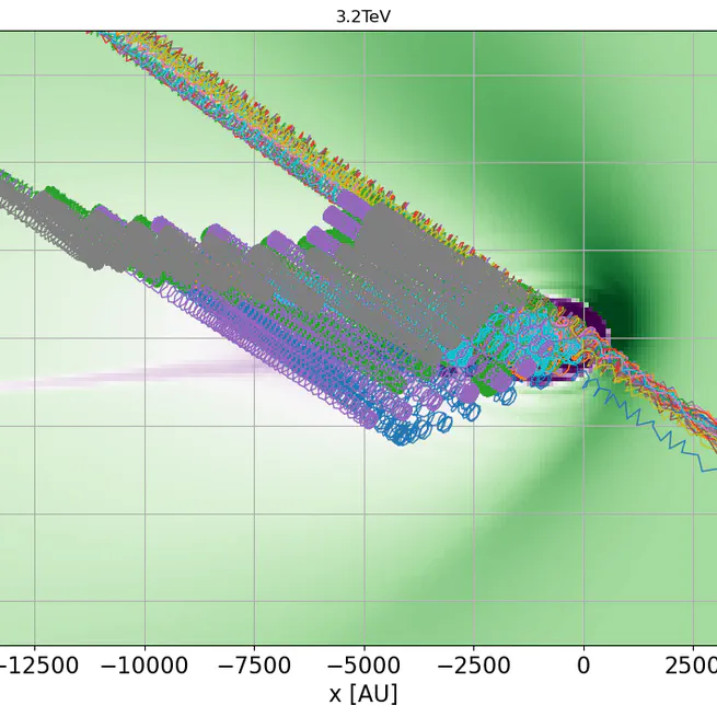
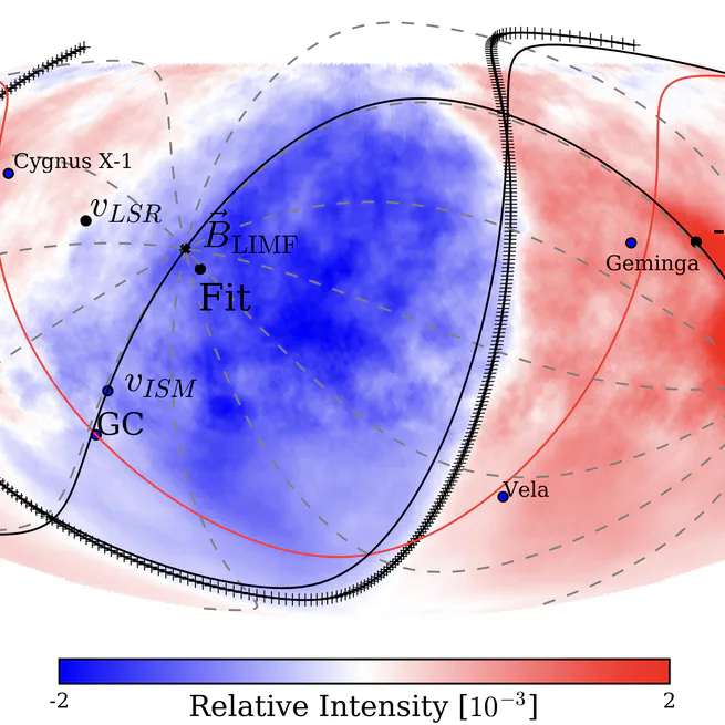
Introduction The propagation of relativistic charged particles in the heliosphere and interstellar magnetic fields is calculated using the ptracing code. This code was originally developed for the studies described in Desiati & Zweibel (2014). It includes several analytical magnetic and electric field configurations and interfaces to different heliospheric numerical models. Additionally, it supports multithreading, allowing it to take full advantage of computers with a large number of CPU cores and shared memory. Trajectories are calculated by numerically integrating the following set of 6–dimensional ordinary differential equations $$\frac{d\mathbf{p}}{dt} = q \left(\mathbf{v}\times\mathbf{B} \right), \, \frac{d\mathbf{r}}{dt} = \mathbf{v},$$ describing the Lorentz force exerted by the magnetic field $\mathbf{B}(\mathbf{r})$ on particles with electric charge $q$ and velocity $\mathbf{v}$, where $\mathbf{r}$ is their position vector and $\mathbf{p}$ the momentum. Momentum is expressed in units of $mc$; $\hat{\mathbf{p}}\equiv\mathbf{p}/mc$. The particle velocity $\mathbf{v}$ is related to $\hat{\mathbf{p}}$ by $\mathbf{v} = \hat{\mathbf{p}}/\sqrt{1+\hat p^2}$ and the particle Lorentz factor $\gamma = \sqrt{1+\hat p^2}$. In these units, the dimensionless particle gyroradius is $\hat r_g = \hat p_{\perp}$, and the dimensionless gyro-frequency is $\hat \omega_g = 1/\gamma$. %We denote normalized variables with a hat. The equations of motion can be numerically integrated using various stepping algorithms. The code supports an adaptive time step size in these calculations, with a tolerance level denoted by a parameter $\epsilon$ to ensure that truncation errors remain sufficiently small. The integration of particle trajectories concludes when either the maximum integration time, $t_\mathrm{max}$, is reached or when the particles have attained a radius of $r_\mathrm{max}$. The figure demonstrates how protons are affected by the heliosphere and the modified magnetic field near its boundary. One challenge in calculating trajectories within open boundary systems is that particles propagating from outside the heliosphere have a very low probability of reaching Earth or passing near it. To address this, we plan to generate 100 million anti-proton trajectories, propagating backward from Earth to a distance of 50,000 AU from the Sun. We compute the trajectories using the Boris Push stepping method. This algorithm has become a standard for this purpose. Although the Boris algorithm is not symplectic, it does conserve phase space volume, and its energy error is globally bounded, comparable to that of symplectic algorithms. To ensure the accuracy of our results and as part of our validation procedure, we will perform additional checks by varying the integration tolerance parameters and comparing the outcomes with the explicit fourth-order Runge-Kutta method. Additionally, we will conduct cross-validation with limited statistics using third-party tools such as CRPropa. We calculate trajectories using heliospheric models provided by our collaborator, Prof. Nikolai Pogorelov, to investigate the systematic effects of model parameters on our data interpretation. According to Liouville’s Theorem, we can interpret the calculated back-propagated anti-proton trajectories as protons traveling from the ISM to Earth. Experimental biases on the heliospheric contribution to the observed TeV cosmic ray anisotropy A preliminary study utilized numerically computed particle trajectories from a computational heliospheric model to assess the experimental biases introduced by ground-based experiments and their impact on interpretations. We intend to conduct thorough investigations into this experimental dimension of cosmic-ray physics, which will aid in developing the analytical tools needed to explore the origins of cosmic-ray anisotropy and its propagation through the interstellar medium and the heliosphere. The paper examines how the heliosphere acts as a magnetic lens that reshapes the TeV cosmic-ray anisotropy we observe on Earth, complicating efforts to infer the true interstellar distribution. Because ground-based reconstructions are effectively “blind” to the north–south (m=0) spherical-harmonic terms, the vertical component of the dipole is lost, which can bias estimates of the pitch-angle distribution in the local interstellar medium (LISM). Even so, the paper argues that higher-order multipoles preserve enough spatial information to constrain the large-scale structure and its alignment with the local interstellar magnetic field (LIMF). The premise is that if we correctly model the heliospheric imprint and account for observational limitations, we can still recover the underlying LISM anisotropy. The reconstructed map of the 10 TeV combined sample after propagation. The direction of the LIMF is indicated by the X and the corresponding magnetic equator (i.e. the plane perpendicular to the uniform LIMF passing by the Earth) is shown with a solid curve. The inferred direction obtained by fitting a circle to the boundary of large-scale excess and deficit regions (dot-dashed green curve) from the true propagated map is indicated with a green star. The equivalent fit (shown as a dashed red curve) for the reconstructed map is indicated with red square. Using back-propagation through a heliospheric field model across multiple rigidities, we reconstruct Earth-frame sky maps, fit the boundary between excess and deficit to infer the LIMF “magnetic equator,” and estimate the missing north–south dipole component. Remapping the result outside the heliosphere then yields an interstellar dipole whose direction is within about 3° of the true LIMF when that compensation is applied (versus ~14° without it). At ~10 TV rigidity, where particle gyroradii match the LIMF draping scale, the heliospheric effect is strong but does not destroy the overall ordering with the LIMF; the method’s accuracy, however, depends on the chosen heliosphere/LIMF model. The paper highlights the next steps, which include scanning heliotail length, solar-cycle phase, turbulence, and LIMF geometry to quantify model sensitivities. Chaotic Behavior of Trapped Cosmic Rays A recently published paper develops a practical way to quantify how cosmic rays behave chaotically when they’re temporarily trapped by coherent magnetic structures—especially the heliosphere acting as a magnetic mirror. Using an axially symmetric “magnetic bottle” tailored to heliospheric scales (field strengths ~1–3 μG; mirror separation ~2000 au), the authors integrate ensembles of 1 TeV test-particle trajectories and compute finite-time Lyapunov exponents (FTLEs), which measure how rapidly nearby trajectories diverge over a chosen time window. They also add time-dependent perturbations designed to mimic solar-cycle polarity reversals (including a check on induced electric fields) to see how temporal variability alters the chaos. The key diagnostic is the joint behavior of FTLE versus a particle’s escape time from the mirror. The central result is a robust power-law correlation: once particles have reached their most chaotic state, the FTLE scales approximately as the inverse of the escape time (slope ≈ −1), and this relation persists under weak and strong time perturbations. On that basis, trajectories naturally fall into regimes—transient (quick escape, little chaos), intermediate (brief explosive divergence), a broad “power-law” class (regular vs. irregular chaotic orbits with steadily increasing dwell times), and, in the unperturbed case only, long-lived trapped orbits. Mapping FTLE and escape time onto the sky reveals distinct regions and gradients in chaoticity; adding perturbations erases the strictly trapped region and redistributes particles toward shorter escape times, while maintaining the same FTLE–escape-time slope. Because 1–10 TV rigidities have gyroradii comparable to heliospheric scales, the study argues that chaotic mirroring can imprint time variability—on solar-cycle timescales and in specific sky sectors—on observed TeV anisotropy maps, such as those from HAWC+IceCube. The method provides a framework for interpreting such variations and is intended to be applied to more realistic MHD–kinetic heliosphere models and to other magnetic mirrors (e.g., superbubbles), thereby linking microphysical trajectory chaos to macroscopic anisotropy morphology.

Aug 17, 2025

Cosmic-ray Anisotropy

Introduction The IceCube and the HAWC observatories have established themselves as leaders in studying Galactic cosmic-ray anisotropy in the TeV–PeV energy range. IceCube captures anisotropy amplitudes with high precision by mapping cosmic-ray arrival directions relative to an isotropic reference. The IceTop surface array detects showers above 500 TeV, while the deep in-ice array records muons down to 10 TeV, both closely aligning with primary cosmic-ray directions. HAWC gamma-ray array detects showers above 1-10 TeV. IceCube and HAWC’s continuous sky observation enhances measurement stability, enabling energy-dependent anisotropy studies and spherical harmonic expansion analysis. Recent findings highlight the dipole component’s amplitude and phase as indicators of cosmic-ray diffusion in interstellar plasma. The angular power spectrum at different energies reflects pitch angle scattering processes. IceCube has submitted results from 12 years (2011–2023) of cosmic-ray muon data, refining event selection for improved stability. High-resolution sky maps will explore temporal anisotropy variations and cross-check muon and shower data consistency. IceCube also analyzes the Compton-Getting effect for calibration and cosmic-ray spectral index measurement. Given individual experiments’ limited sky coverage, full-sky measurements via collaborations with HAWC, GRAPES-3, TALE, and KASCADE aim to provide a comprehensive view of anisotropy. These efforts will improve understanding of cosmic-ray diffusion and heliospheric influence on observed distributions. Publications This is the list of cosmic-ray anisotropy results published by the team: citation title DOI arXiv ApJ (2010) 718 L194 Measurement of the Anisotropy of Cosmic Ray Arrival Directions with IceCube 10.1088/2041-8205/718/2/L194 1005.2960 ApJ (2011) 740 16 Observation of Anisotropy in the Arrival Directions of Galactic Cosmic Rays at Multiple Angular Scales with IceCube 10.1088/0004-637X/740/1/16 1105.2326 ApJ (2012) 746 33 Observation of an Anisotropy in the Galactic Cosmic Ray arrival direction at 400 TeV with IceCube 10.1088/0004-637X/746/1/33 1109.1017 ApJ (2013) 765 55 Observation of Cosmic Ray Anisotropy with the IceTop Air Shower Array 10.1088/0004-637X/765/1/55 1210.5278 ApJ (2016) 826 220 Anisotropy in Cosmic-Ray Arrival Directions in the Southern Hemisphere with Six Years of Data from the IceCube Detector 10.3847/0004-637X/826/2/220 1603.01227 ApJ (2019) 871 96 All-Sky Measurement of the Anisotropy of Cosmic Rays at 10 TeV and Mapping of the Local Interstellar Magnetic Field 10.3847/1538-4357/aaf5cc 1812.05682 ApJ (2025) 981 182 Observation of Cosmic-Ray Anisotropy in the Southern Hemisphere with 12 yr of Data Collected by the IceCube Neutrino Observatory 10.3847/1538-4357/adb1de 2412.05046 Observation of Cosmic-Ray Anisotropy in the Southern Hemisphere with 12 yr of Data Collected by the IceCube Neutrino Observatory In our latest IceCube publication, we report a definitive, high-statistics view of TeV–PeV cosmic-ray anisotropy in the Southern Hemisphere using 7.92×10¹¹ cosmic-ray–induced muon events collected by the fully built detector between May 13, 2011 and May 12, 2023. With improved simulations and uniform, year-by-year processing, systematic uncertainties are reduced to levels below statistical fluctuations. The data confirm the long-noted evolution of the anisotropy’s angular structure between ~10 TeV and 1 PeV—most prominently across 100–300 TeV—and, for the first time in IceCube, present energy-dependent angular power spectra that show comparatively diminished large-scale power at the highest energies while retaining significant medium/small-scale structure down to ~6°. Methodologically, the analysis builds reference maps via 24-hour time-scrambling and quantifies relative intensity per sky pixel, with top-hat smoothing (typically 20°; 5° for certain low-energy residual maps) used only for visualization; the median angular resolution is ~3° and reaches ~1° above 100 TeV. Systematics from the interference between sidereal anisotropy and the solar Compton–Getting effect are controlled by analyzing full calendar years and by checking the antisidereal frame; the resulting systematic spreads are now comparable to statistical errors—a marked improvement over earlier IceCube work. Angular pseudo-power for selected spherical harmonic modes (ℓ) as a function of median primary energy for 12 yr of IceCube data. Errors bars are statistical. The bands indicate the 95% spread in C˜ℓ from a large sample of scrambled maps. The color of the bands corresponds to that of the data symbols but in a lighter shade. Physically, the horizontal (equatorial) dipole component behaves as in other experiments: its amplitude decreases from ~10 TeV to just above 100 TeV—reaching a minimum of ≈2×10⁻⁴ while its phase flips from ~RA 50° to ~RA 260°—then rises again with energy. At ~5.3 PeV, the dipole is only marginally distinguishable from isotropy, yielding a 99%-CL upper limit of 3.34×10⁻³. The measured dipole phase and amplitude align with Northern-hemisphere results once field-of-view biases in one-dimensional fits are corrected, reinforcing a coherent, largely horizontal large-scale pattern across both hemispheres. IceCube’s event selection and reconstruction underpin these results: the detector triggers at 2.0–2.3 kHz on muon bundles that track the parent cosmic-ray directions to within a few degrees, and a compact “DST” data stream preserves the essential kinematics for anisotropy analyses over the full 12-year exposure. Residual maps—after subtracting dipole and quadrupole—reveal persistent smaller-scale structure at both low (<18 TeV) and high (>320 TeV) energies. Together, these advances deliver the most precise Southern-sky anisotropy maps to date and a clean baseline for future joint, full-sky studies that probe how the anisotropy’s scale mix evolves with energy.

Aug 17, 2025

Using TeV Cosmic Rays to probe the Heliosphere's Boundary with the Local Interstellar Medium

The outer heliosphere regulates cosmic ray penetration into near-Earth space, reduces space radiation, and makes life possible in our solar system. Voyager and IBEX in-situ and remote observations of the outer heliosphere and the distorted local interstellar magnetic are important for heliospheric modeling. TeV cosmic rays provide a new tool to study the heliosphere interstellar medium boundary.

Jul 1, 2023